7 minutes
Constraint Solvers and Z3
A constraint solver must be versatile, that is, it should be able to act as an:
- Interpreter: Given the input, solve for the output of the equation.
- Inverter: Given the output, solve for the input of the equation.
- Synthesizer: Act as both Interpreter and Inverter.
Formulating Programs
Assume a formula 𝑆ₚ(𝑥, 𝑦) which holds if and only if program P(x) outputs value y such that:
Program: f(𝑥) { return 𝑥 + 𝑥 }
Formula: 𝑆𝒻(𝑥, 𝑦) : 𝑦 = 𝑥 + 𝑥
Now, with the program represented as a formula, the solver can be versatile.
Solver as an Interpreter:
Given x, evaluate f(x).
𝑆𝒻(𝑥, 𝑦) ∧ 𝑥 = 3
⇨ 𝑦 ↦ 6
Solver as an Inverter:
Given f(x), find x.
𝑆𝒻(𝑥, 𝑦) ∧ 𝑦 = 6
⇨ 𝑥 ↦ 3
This solver “bidirectionality” enables Synthesis.
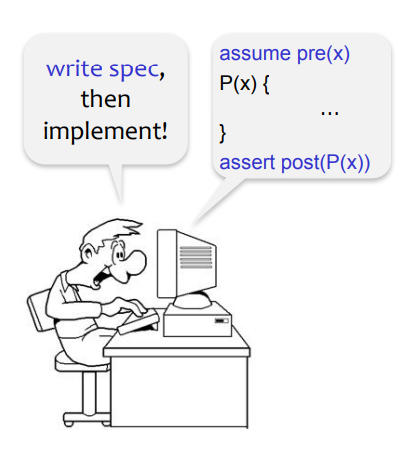
Specifications
A predicate is a binary-valued function of non-binary variables.
Precondition (denoted 𝑝𝑟𝑒(𝑥)) of a procedure f is a predicate over f’s parameters 𝑥 that always holds when f is called. Therefore, f can assume that 𝑝𝑟𝑒(𝑥) holds.
Postcondition (denoted 𝑝𝑜𝑠𝑡(𝑥, 𝑦)) is a predicate over parameters of f and its return value 𝑦 that holds when f returns. Therefore, f ensures that 𝑝𝑜𝑠𝑡(𝑥, 𝑦) holds.
These pre and post-conditions are known as Contracts.
Usually, these contracts are tested (that is, evaluated dynamically, during execution).
 Contracts tested during execution.
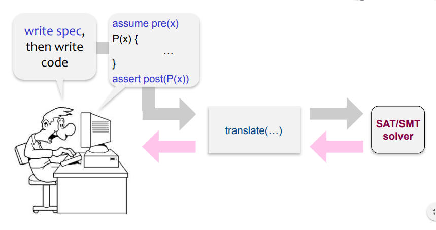
However, with solvers, we want to test these contracts statically, at design time.
 Contracts tested during design with solvers.
Verification Problem
 Verification with Constraint Solver.
The problem at hand is to basically translate preconditions, postconditions, loop conditions, and assertions into solver’s formulae in order to determine/verify if all properties can hold.
Correctness condition 𝜙 says that the program is correct for all valid inputs:
∀𝑥 . 𝑝𝑟𝑒(𝑥) ⇒ 𝑆ₚ(𝑥, 𝑦) ∧ 𝑝𝑜𝑠𝑡(𝑥, 𝑦)
where, 𝑝𝑟𝑒(𝑥) is valid for all 𝑥.
𝑆ₚ(𝑥, 𝑦) computes 𝑦 from 𝑥.
𝑝𝑜𝑠𝑡(𝑥, 𝑦) is correct.
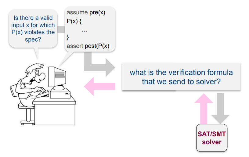
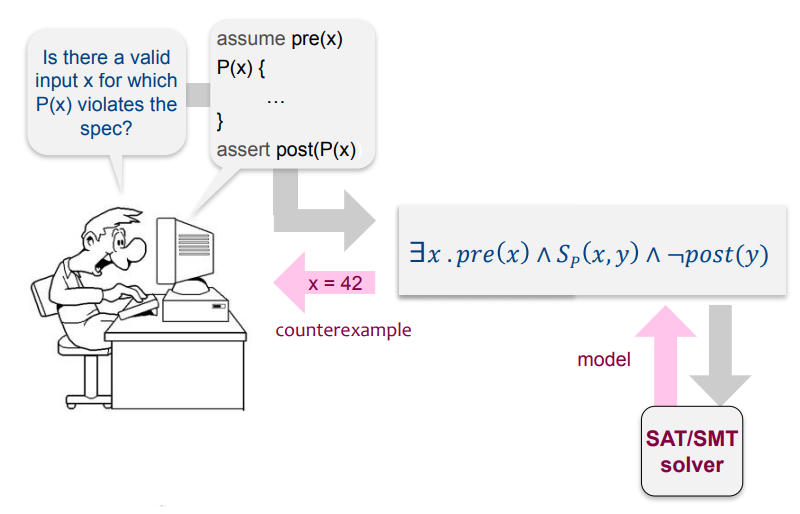
To prove correctness for all inputs 𝑥, search for counterexample 𝑥 where 𝜙 does not hold:
¬ (∀𝑥 . 𝑝𝑟𝑒(𝑥) ⇒ 𝑆ₚ(𝑥, 𝑦) ∧ 𝑝𝑜𝑠𝑡(𝑥, 𝑦))
⇨ ∃𝑥 . ¬ 𝑝𝑟𝑒(𝑥) ⇒ 𝑆ₚ(𝑥, 𝑦) ∧ 𝑝𝑜𝑠𝑡(𝑥, 𝑦)
⇨ ∃𝑥 . 𝑝𝑟𝑒(𝑥) ∧ ¬ 𝑆ₚ(𝑥, 𝑦) ∧ 𝑝𝑜𝑠𝑡(𝑥, 𝑦)
Since 𝑆ₚ always holds, as we can always find 𝑦 given 𝑥,
⇨ ∃𝑥 . 𝑝𝑟𝑒(𝑥) ∧ 𝑆ₚ(𝑥, 𝑦) ∧ ¬ 𝑝𝑜𝑠𝑡(𝑥, 𝑦)
 Passing the verification condition to the solver.
SAT Solver
A formula/constraint F is satisfiable if there is some assignment of appropriate values to its uninterpreted symbols under which F evaluates to true. Thus, the language of SAT Solvers is Boolean logic.
A Satisfiability Solver accepts a formula 𝜙(𝑥, 𝑦, 𝑧) and checks if 𝜙 is satisfiable (SAT).
If yes, the solver returns a model m, a valuation of 𝑥, 𝑦, 𝑧 that satisfies 𝜙, ie, 𝑚 makes 𝜙 true. If the formula is unsatisfiable (UNSAT), some solvers return minimal unsat core of 𝜙, a smallest set of clauses of 𝜙 that cannot be satisfied.
Such problems are typically in the CNF(Conjuctive Normal Form) form, that is, a conjunction of one or more clauses, where a clause is a disjunction of literals (an AND of ORs).
SAT solvers are automatic and efficient. As a result, they are frequently used as the “engine” behind verification applications.
SMT Solver
The Satisfiability Modulo Theories problem is a decision problem for logical formulas with respect to combinations of background theories expressed in classical first-order logic with equality.
- Modular Theory implies that the solver is extensible with different theories.
In simpler words, SMT Solvers are built on top of SAT solvers, and they are able to combine the powers of the SAT solver with other domain specific theory solvers(the extensible property comes in here) to solve NP complete problems. Thus, SMT Solvers rely on our ability to solve satisfiability problems, to take problems with boolean variables and constraints to tell us whether there is an assignment to these variables that satisfies that particular problem. A SAT Solver then tries random assignments and propagates them through the constraints. When it runs into a contradiction, it analyses the set of limitations that led to the contradiction and summarizes them into a new constraint so that the same problem can be avoided next time onwards.
For example, say a stage is given:
x>5 AND y<5 AND (y>x OR y>2)
SMT solver will divide it into domain specific theories.
⇨ |x>5| AND |y<5| AND (|y>x| OR |y>2|) // Linear Arithmetic Theory and Boolean Logic.
⇨ f1 AND f2 AND (f3 OR f4)
And then hands it off to a SAT Solver, which will try to make this stage satisfiable.
Let’s say it comes up with the conclusion that making f1, f2 and f3 true will make it satisfiable.
Then domain specific theory solvers (Linear Arithmetic Solver) solves f1, f2 and f3 so as to find inputs that make them satisfiable. Thus it becomes a purely linear arithmetic question now, with no boolean logic.
This specific solver can imply different traditional techniques such as simplex methods to solve these systems for linear inequalities, etc. This solver quickly returns that this conclusion is unsatisfiable, and returns the result along with an explanation to the SAT solver (that f1, f2 and f3 are mutually exclusive). SAT Solver then remembers not to try that particular situtation anymore. It then comes up with the conclusion that making f1, f2 and f4 true will make the situation satisfiable. This time the specific solver returns satisfiable, thus bringing this situation to a “satisfiable” conclusion.
Since systems are usually designed and modeled at a higher level than the Boolean level, the translation to Boolean logic can be expensive. SMT Solvers therefore aim to create verification engines that can reason natively at a higher level of abstraction while retaining the efficiency of SAT Solvers. The language of SMT Solvers is therefore First-Order-Logic. The language includes the Boolean operations of Boolean logic, but instead of propositional variables, more complicated expressions involving constant, function, and predicate symbols are used. In other words, imagine an instance of the Boolean satisfiability problem (SAT) in which some of the binary variables are replaced by predicates over a suitable set of non-binary variables.
Some of the popular theories are:
- Bit Vector Theory
- Using bit vectors of fixed bit width, such as 8bit vectors and 32bit vectors, as symbols.
- Theory of Arrays
- Used for a collection of objects where the size of an object is unknown beforehand, such as strings.
- Theory of Integer Arithmetic
- Symbols are limited to the integral domain.
- Theory of Uninterpreted Functions
- Within a formula, a call to a function is made, which we know nothing about, except the fact that it will always give the same output for a given input value, such as square root.
A very popular SMT Solver is Z3.
Z3
Introducing the powers of Z3 in python, run pip install z3-solver to install it via pip.
Follow archived docs for basic syntax and a jump start.
Official Docs for reference to the API in different languages.
Taking Z3 for a spin, let’s tackle a well-known problem: Sudoku Solver.
Read this page implemented in this IPython Notebook for a comprehensive explanation on a Sudoku Solver.
Using Z3 for binary analysis, let’s analyse a binary.
Taking up a serial validator, let’s take a look at the binary’s decompilation.
We are looking at the decompilation to save ourselves the time and effort of reverse engineering, since the main focus is to demonstrate the usage of Z3 to resolve a serial check.
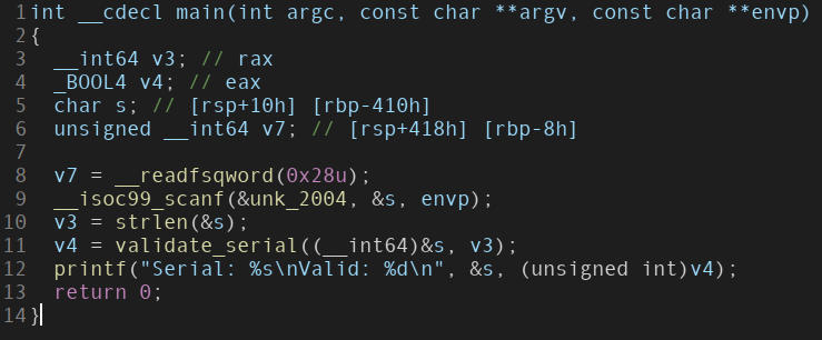 “main” function.
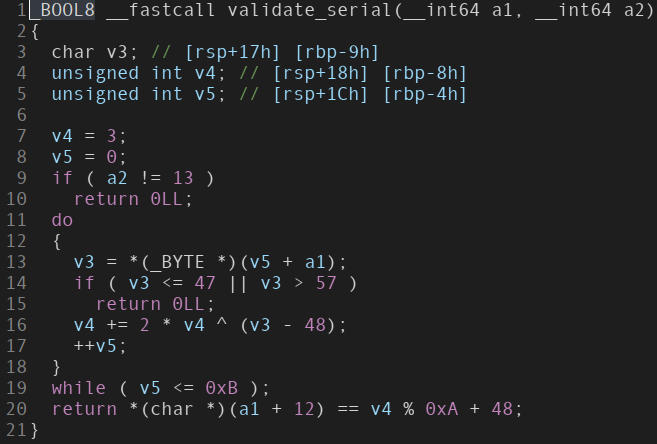 “validate_serial” function.
Examining the validate_serial function, it is clear that
- Serial is passed in
a1. - Length of the serial is 13, passed in
a2. v5is the iterator for the loop run ona1. Loop runs till the last element, but not on last element since it’s an exit controlled loop using a pre-increment operator.- All values in
a1should be between 46 and 57(line 14), which then has 48 subtracted from it(line 16). Even out to values between 0 and 9(both inclusive). v4is a running sum, with an initial value of 3. Only uses previous value and serial digit value to update current value.- Returns boolean value, so the target is to get the output as
Valid: 1.
Using the constraints and computations specified, we’ll write a Z3 script to give us our good serial.
Read this page implemented in this IPython Notebook to follow the solution for this problem.
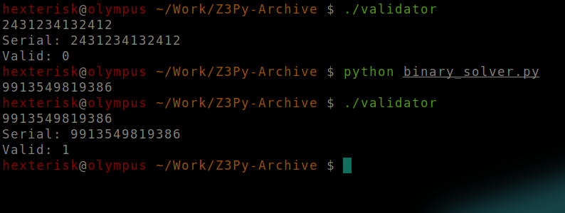 Output.
Credits for the guidance to Calle Svensson’s talk “SMT in reverse engineering, for dummies” at SEC-T 0x09.