8 minutes
Binary Instrumentation
Inserting new code at any point in an existing binary to observe or modify the binary’s behavior in some way is called instrumenting the binary. The point where you add new code is called the instrumentation point, and the added code is called instrumentation code.
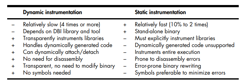 Tradeoffs of Dynamic and Static Binary Instrumentation.
Static Binary Instrumentation
Static Binary Instrumentation works by disassembling a binary and then adding instrumentation code where needed and storing the updated binary permanently on disk.
Naive Implementation
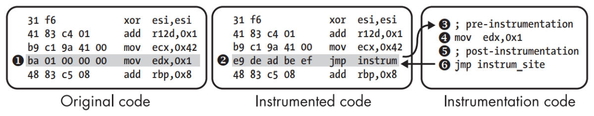 A nongeneric SBI approach that uses jmp to hook instrumentation points.
Instrumenting the instruction ➊, add instrumentation code to run before and after that instruction. Overwrite it with a jmp to your instrumentation code ➋, stored in a separate code section or library. The instrumentation code runs any pre-instrumentation code ➌, the original instruction ➍ and then the post-instrumentation code ➎. Finally, the instrumentation code jumps back to the instruction following the instrumentation point ➏, resuming normal execution.
The issue is that a jmp instruction is 5-bytes, 1 opcode byte with a 32-bit offset. Replacing an instruction with a smaller byte-length will overwrite following bytes, such as instrumenting a xor esi,esi (2-bytes) would require replacing it with a 5-byte jmp.
int3 Approach
The x86 int3 instruction generates a software interrupt that are caught as (on Linux) SIGTRAP signals. It’s only 1 byte long, so any instruction can be overwritten with it. On SIGTRAP, use Linux’s ptrace API to find out at which address the interrupt occurred, telling you the instrumentation point address. You can then invoke the appropriate instrumentation code for that instrumentation point.
Trampoline Approach
Direct Calls
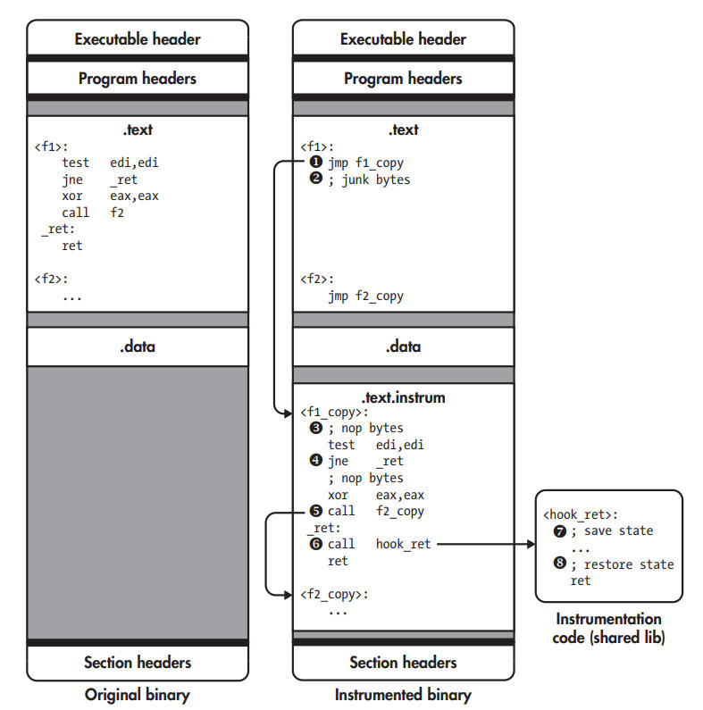 Static binary instrumentation with trampolines.
SBI engine creates copies of all the original functions, places them in a new code section, and overwrites the first instruction of each original function with jmp instructions called trampolines to redirect the original code to the instrumented copy. Whenever a call or jump transfers control to a part of the original code, the trampoline at that location immediately jumps to the corresponding instrumented code. Instruction jmp is 5-bytes, so it may partially overwrite and corrupt multiple instructions, creating junk bytes right after the trampoline. It isn’t a problem since these corrupted instructions are never executed.
As soon as f1 is called, the trampoline jumps to f1_copy ➊, the instrumented version of f1. Junk bytes at ➋ aren’t executed. SBI engine inserts several nop in f1_copy ➌ so that to instrument an instruction, the SBI engine can simply overwrite the nop at that instrumentation point with a jmp or call to a chunk of instrumentation code. In the figure, all nop regions are unused except for the last one, just before the ret. SBI engine patches the offsets of all relative jmp, and replaces all 2-byte relative jmp having an 8-bit offset with a corresponding 5-byte version that has a 32-bit offset ➍ as the offset between jmp and their targets may become too large to encode in 8 bits. SBI engine rewrites direct calls too, such as call f2 so that they target the instrumented function instead of the original ➎. Trampolines are needed at the start of every original function to accommodate indirect calls. For the engine instrumenting every ret, it overwrites the nop reserved for this purpose with a jmp or call to the instrumentation code ➏, hook_ret, which is placed in a shared library and reached by a call that the SBI engine placed at the instrumentation point, first saves state ➐, such as register contents, and then runs any instrumentation code that you specified. Finally, it restores the saved state ➑ and resumes normal execution by returning to the instruction following the instrumentation point.
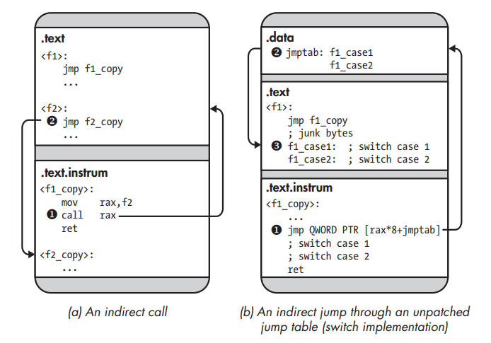 Indirect control transfers in a statically instrumented binary.
Indirect Calls
The SBI engine doesn’t alter code that computes addresses, so the target addresses used by indirect calls point to the original function ➊. Because there’s a trampoline at the start of every original function, control flows immediately back to the instrumented version of the function ➋.
At the binary level, switch statements are often implemented using a jump table that contains all the addresses of the possible switch cases. The switch computes the corresponding jump table index and uses an indirect jmp to jump to the address stored there ➊. The addresses stored in the jump table all point into the original code ➋. Thus, the indirect jmp ends up in the middle of an original function, where there’s no trampoline, and resumes execution there ➌. To avoid this problem, the SBI engine must either patch the jump table, changing original code addresses to new ones, or place a trampoline at every switch case in the original code. Unfortunately, basic symbolic information (as opposed to extensive DWARF information) contains no information on the layout of switch statements, making it hard to figure out where to place the trampolines. Additionally, there may not be enough room between the switch statements to accommodate all trampolines. Patching jump tables is also dangerous because you risk erroneously changing data that just happens to be a valid address but isn’t really part of a jump table.
Reliability
- Error-prone.
- Programs may (however unlikely) contain very short functions that don’t have enough room for a 5-byte jmp, requiring the SBI engine to fall back to another solution like the int 3 approach.
- If the binary contains any inline data mixed in with the code, trampolines may inadvertently overwrite part of that data, causing errors when the program uses the data.
- All this is assuming that the disassembly used is correct in the first place; if it’s not, any changes made by the SBI engine may break the binary.
PIE
- On 32-bit x86, PIE binaries read the program counter by executing a call instruction and then reading the return address from the stack.
// copies the return address into ebx and then returns.
<__x86.get_pc_thunk.bx>:
	mov ebx,DWORD PTR [esp]
	ret
- On x64, you can read the program counter (rip) directly.
- The danger with PIE binaries is that they may read the program counter while running instrumented code and use it in address computations. This likely yields incorrect results because the layout of the instrumented code differs from the original layout that the address computation assumes. SBI engines solve this problem using instrument code constructs that read the program counter such that they return the value the program counter would have in the original code. That way, subsequent address computations yield the original code location just as in an uninstrumented binary, allowing the SBI engine to intercept control there with a trampoline.
Dynamic Binary Instrumentation
DBI engines monitor binaries (or rather, processes) as they execute and instrument the instruction stream. They don’t require disassembly or binary rewriting, making them less error-prone.
Architecture
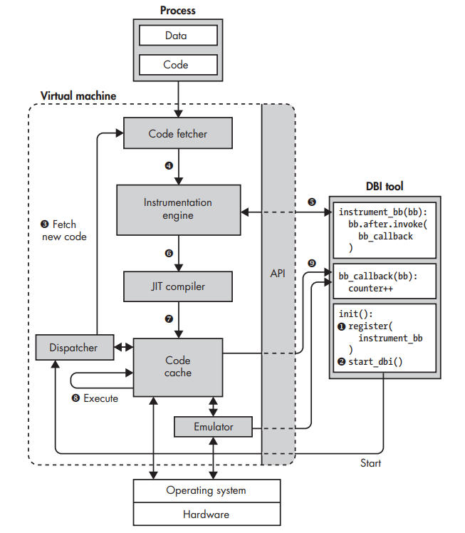 Architecture of a DBI system.
The DBI engine exposes an API that allows you to write user-defined DBI tools (often in the form of a shared library loaded by the engine) that specify which code should be instrumented and how. For example, the DBI tool shown on the right side implements (in pseudocode) a simple profiler that counts how many basic blocks are executed. To achieve that, it uses the DBI engine’s API to instrument the last instruction of every basic block with a callback to a function that increments a counter.
DBI tool’s initialization function registers a function called instrument_bb with the DBI engine ➊. This function tells the DBI engine how to instrument every basic block; in this case, it adds a callback to bb_callback after the last instruction in the basic block. The DBI engine then starts the application ➋. The DBI engine never runs the application process directly but instead runs code in a code cache that contains all the instrumented code. Initially, the code cache is empty, so the DBI engine fetches a block of code from the process ➌ and instruments that code ➍ as instructed by the DBI tool ➎. Assuming the engine instruments code at basic block granularity (not always) JIT compiler ➏, which re-optimizes the instrumented code and stores the compiled code in the code cache ➐. The JIT compiler also rewrites control flow instructions to ensure that the DBI engine retains control, preventing control transfers from continuing execution in the uninstrumented application process.
This instrumented and JIT-compiled code now executes in the code cache until there’s a control-flow instruction that requires fetching new code or looking up another code chunk in the cache ➑. The instrumented code contains callbacks to functions in the DBI tool that observe or modify the code’s behavior ➒.
- The JIT compiler in a DBI engine doesn’t translate the code into a different language; it compiles from native machine code to native machine code. It’s only necessary to instrument and JIT-compile code the first time it’s executed.
- DBI engines like Pin and DynamoRIO reduce runtime overhead by rewriting control-flow instructions when possible, so they jump directly to the next block in the code cache without mediation by the DBI engine. When that’s not possible (for example, for indirect calls), the rewritten instructions return control to the DBI engine so that it can prepare and start the next code chunk. While most instructions run natively in the code cache, the DBI engine may emulate some instructions instead of running them directly. For example, Pin does this for system calls like execve that require special handling by the DBI engine.
Citation: Practical Binary Analysis.