19 minutes
Disassembly and Binary Analysis Fundamentals
Static Disassembly
When people say disassembly, they usually mean static disassembly, which involves extracting the instructions from a binary without executing it.
Linear Disassembly
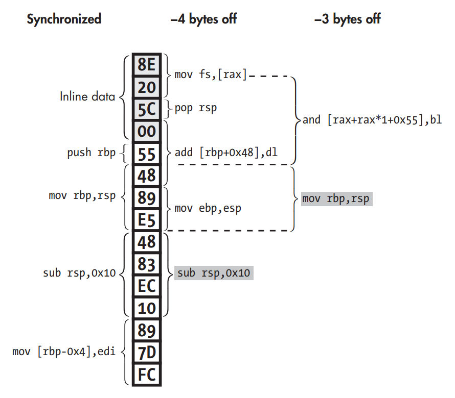 Disassembly desynchronization due to inline data interpreted as code. The instruction where the disassembly resynchronizes is shaded gray.
- It iterates through all code segments in a binary, decoding all bytes consecutively and parsing them into a list of instructions. Many simple disassemblers, including objdump, use this approach.
- The risk is that not all bytes may be instructions.
- Some compilers like Visual Studio intersperse data such as jump tables with the code, without leaving any clues as to where exactly that data is. If disassemblers accidentally parse this inline data as code, they may encounter invalid opcodes. Even worse, the data bytes may coincidentally correspond to valid opcodes, leading the disassembler to output bogus instructions. This is especially likely on dense ISAs like x86, where most byte values represent a valid opcode.
- On ISAs with variable-length opcodes such as x86, inline data may even cause the disassembler to become desynchronized with respect to the true instruction stream. Though the disassembler will typically self-resynchronize, desynchronization can cause the first few real instructions following inline data to be missed.
Recursive Disassembly
- Sensitive to control flow, it starts from known entry points into the binary (such as the main entry point and exported function symbols) and from there recursively follows control flow (such as jumps and calls) to discover code. This allows recursive disassembly to work around data bytes in all but a handful of corner cases.
- To maximize code coverage, recursive disassemblers typically assume that the bytes directly after a call instruction must also be disassembled since they are the most likely target of an eventual ret. Additionally, disassemblers assume that both edges of a conditional jump target valid instructions. Both of these assumptions may be violated in rare cases, such as in deliberately obfuscated binaries.
- The downside of this approach is that not all control flow is so easy to follow. For instance, it’s often difficult, if not impossible, to statically figure out the possible targets of indirect jumps or calls. As a result, the disassembler may miss blocks of code, or even entire functions, targeted by indirect jumps or calls, unless it uses special heuristics to resolve the control flow. For example, jump tables make recursive disassembly more difficult because they use indirect control flow.
Dynamic Disassembly
Dynamic disassembly, more commonly known as execution tracing, logs each executed instruction as the binary runs.
- Dynamic analysis solves many of the problems with static disassembly because it has a rich set of runtime information at its disposal, such as concrete register and memory contents. Thus dynamic disassemblers, also known as execution tracers or instruction tracers, may simply dump instructions (and possibly memory/register contents) as the program executes.
- When execution reaches a particular address, you can be absolutely sure there’s an instruction there, so dynamic disassembly doesn’t suffer from the inaccuracy problems involved with resolving indirect calls in static disassembly.
- The main disadvantage of all dynamic analysis is the code coverage problem: the analysis only ever sees the instructions that are actually executed during the analysis run. Thus, if any crucial information is hidden in other instructions, the analysis will never know about it.
Fuzzers
Tools that try to automatically generate inputs to cover new code paths in a given binary.
- Generation-based fuzzers: These generate inputs from scratch (possibly with knowledge of the expected input format).
- Mutation-based fuzzers: These fuzzers generate new inputs by mutating known valid inputs in some way, for instance, starting from an existing test suite.
Symbolic Execution
- At each point in the execution, every CPU register and memory area contains some particular value, and these values change over time as the application’s computation proceeds. Symbolic execution allows you to execute an application not with concrete values but with symbolic values. You can think of symbolic values as mathematical symbols. A symbolic execution is essentially an emulation of a program, where all or some of the variables (or register and memory states) are represented using such symbols.
- Basically initializing variables with symbolic values like α instead of numeric values and then computing path constraints. which are just restrictions on the concrete values that the symbols could take, given the branches that have been traversed so far.
- The key point is that given the list of path constraints, you can check whether there’s any concrete input that would satisfy all these constraints. There are special programs, called constraint solvers, that check, given a list of constraints, whether there’s any way to satisfy these constraints.
- Helps with code coverage problem by adjusting path constraints for the solver.
Structuring Disassembled Code and Data
Large unstructured heaps of disassembled instructions are nearly impossible to analyze, so most disassemblers structure the disassembled code in some way that’s easier to analyze. Two ways:
- Compartmentalizing: By breaking the code into logically connected chunks, it becomes easier to analyze what each chunk does and how chunks of code relate to each other.
- Revealing control flow: Some of the code structures I’ll discuss next explicitly represent not only the code itself but also the control transfers between blocks of code. These structures can be represented visually, making it much easier to quickly see how control flows through the code and to get a quick idea of what the code does.
- Most disassemblers make some effort to recover the original program’s function structure and use it to group disassembled instructions by function. This is known as function detection. Not only does function detection make the code much easier to understand for human reverse engineers, but it also helps in automated analysis.
- For binaries with symbolic information, function detection is trivial; the symbol table specifies the set of functions, along with their names, start addresses, and sizes.
- Stripped binaries have functions with no real meaning at the binary level, so their boundaries may become blurred during compilation. The code belonging to a particular function might not even be arranged contiguously in the binary. Bits and pieces of the function might be scattered throughout the code section, and chunks of code may even be shared between functions (known as overlapping code blocks).
- The predominant strategy that disassemblers use for function detection is based on function signatures, which are patterns of instructions often used at the start or end of a function.
- Done by recursive disassemblers.
- Linear disassemblers don’t do function detection except when symbols are available.
- Function signature patterns include well-known function prologues (instructions used to set up the function’s stack frame) and function epilogues (used to tear down the stack frame).
Control Flow Graphs
 CFG as seen in IDA Pro.
- Control Flow Graphs (CFGs) offer a convenient graphical representation of the code structure, which makes it easy to understand a function’s structure.
- CFGs represent the code inside a function as a set of code blocks, called basic blocks, connected by branch edges, shown here as arrows. A basic block is a sequence of instructions, where the first instruction is the only entry point (the only instruction targeted by any jump in the binary), and the last instruction is the only exit point (the only instruction in the sequence that may jump to another basic block).
- Disassemblers often omit indirect edges from the CFG because it’s difficult to resolve the potential targets of such edges statically. Disassemblers also sometimes define a global CFG rather than per-function CFGs. Such a global CFG is called an interprocedural CFG (ICFG) since it’s essentially the union of all per-function CFGs (procedure is another word for function). ICFGs avoid the need for error-prone function detection but don’t offer the compartmentalization benefits that per-function CFGs have.
Call Graphs
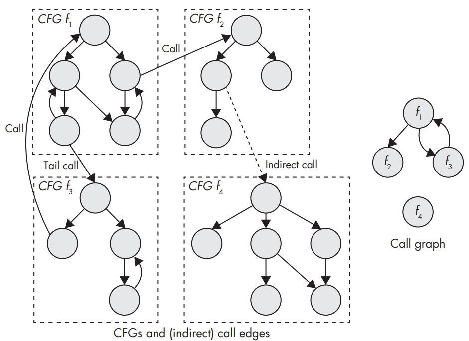 CFGs and connections between functions (left) and the corresponding call graph (right).
- Call graphs show you which functions may call each other. They show the relationship between call sites and functions.
- They often omit indirect call edges because it’s infeasible to accurately figure out which functions may be called by a given indirect call site.
- Functions whose address is stored by some instruction from .text section are called address-taken functions. They might be called indirectly, even if you don’t know exactly by which call site. If a function’s address is never taken and doesn’t appear in any data sections, you know it will never be called indirectly.
- Considering procedural languages and object oriented code, compilers emit tables of function pointers, called vtables, that contain pointers to all the virtual functions of a particular class. Vtables are usually kept in read-only memory, and each polymorphic object has a pointer vptr to the vtable for the object’s type. To invoke a virtual method, the compiler emits code that follows the object’s vptr at runtime and indirectly calls the correct entry in its vtable.
Data Structures
- Automatic data structure detection in stripped binaries is a notoriously difficult problem. But there are some exceptions:
- If a reference to a data object is passed to a well-known function, such as a library function, some disassemblers can automatically infer the data type based on the specification of the library function.
- Primitive types can sometimes be inferred by the registers they’re kept in or the instructions used to manipulate the data. For instance, if you see a floating-point register or instruction being used, you know the data in question is a floating-point number. If you see a lodsb (load string byte) or stosb (store string byte) instruction, it’s likely manipulating a string.
- For composite types such as struct types or arrays, all bets are off, and you’ll have to rely on your own analysis.
Intermediate Representations
- The sheer number of instructions and side effects makes it difficult to reason about binary programs in an automated way, like add on x86 have side effects, such as setting status flags in the eflags register.
- Intermediate representations (IR), also known as intermediate languages, are designed to remove this burden. An IR is a simple language that serves as an abstraction from low-level machine languages like x86 and ARM.
- The idea of IR languages is to automatically translate real machine code, such as x86 code, into an IR that captures all of the machine code’s semantics but is much simpler to analyze. For comparison, REIL contains only 17 different instructions, as opposed to x86’s hundreds of instructions. Moreover, languages like REIL, VEX and LLVM IR explicitly express all operations, with no obscure instruction side effects.
- It’s still a lot of work to implement the translation step from low-level machine code to IR code, but once that work is done, it’s much easier to implement new binary analyses on top of the translated code. Instead of having to write instruction-specific handlers for every binary analysis, with IRs you only have to do that once to implement the translation step. Moreover, you can write translators for many ISAs, such as x86, ARM, and MIPS, and map them all onto the same IR. That way, any binary analysis tool that works on that IR automatically inherits support for all of the ISAs that the IR supports.
- The trade-off of translating a complex instruction set like x86 into a simple language like REIL, VEX, or LLVM IR is that IR languages are far less concise. That’s an inherent result of expressing complex operations, including all side effects, with a limited number of simple instructions. This is generally not an issue for automated analyses, but it does tend to make intermediate representations hard to read for humans.
- Translation of the x86-64 instruction add rax,rdx into VEX IR:
➊ IRSB {
➋ t0:Ity_I64 t1:Ity_I64 t2:Ity_I64 t3:Ity_I64
➌ 00 | ------ IMark(0x40339f, 3, 0) ------
➍ 01 | t2 = GET:I64(rax)
02 | t1 = GET:I64(rdx)
➎ 03 | t0 = Add64(t2,t1)
➏ 04 | PUT(cc_op) = 0x0000000000000004
05 | PUT(cc_dep1) = t2
06 | PUT(cc_dep2) = t1
➐ 07 | PUT(rax) = t0
➑ 08 | PUT(pc) = 0x00000000004033a2
09 | t3 = GET:I64(pc)
➒ NEXT: PUT(rip) = t3; Ijk_Boring
}
As you can see, the single add instruction results in 10 VEX instructions, plus some metadata. First, there’s some metadata that says this is an IR super block (IRSB) ➊ corresponding to one machine instruction. The IRSB contains four temporary values labeled t0–t3, all of type Ity_I64 (64-bit integer) ➋. Then there’s an IMark ➌, which is metadata stating the machine instruction’s address and length, among other things. Next come the actual IR instructions modeling the add. First, there are two GET instructions that fetch 64-bit values from rax and rdx into temporary stores t2 and t1, respectively ➍. Note that, here, rax and rdx are just symbolic names for the parts of VEX’s state used to model these registers—the VEX instructions don’t fetch from the real rax or rdx registers but rather from VEX’s mirror state of those registers. To perform the actual addition, the IR uses VEX’s Add64 instruction, adding the two 64-bit integers t2 and t1 and storing the result in t0 ➎. After the addition, there are some PUT instructions that model the add instruction’s side effects, such as updating the x86 status flags ➏. Then, another PUT stores the result of the addition into VEX’s state representing rax ➐. Finally, the VEX IR models updating the program counter to the next instruction ➑. The Ijk_Boring (Jump Kind Boring) ➒ is a control-flow hint that says the add instruction doesn’t affect the control flow in any interesting way; since the add isn’t a branch of any kind, control just “falls through” to the next instruction in memory. In contrast, branch instructions can be marked with hints like Ijk_Call or Ijk_Ret to inform the analysis that a call or return is taking place, for example.
Fundamental Analysis Methods
A few standard analysis that are widely applicable and aren’t stand-alone binary analysis techniques, but can be used as ingredients of more advanced binary analysis.
Binary Analysis Properties
Some of the different properties that any binary analysis approach can have that will help to classify the different techniques:
Interprocedural and Intraprocedural Analysis
- The number of possible paths through a program increases exponentially with the number of control transfers (such as jumps and calls) in the program.
- An Intraprocedural Analysis will analyze the CFG of each function in turn. The downside is that it’s incomplete, for instance:
- If your program contains a bug that’s triggered only after a very specific combination of function calls, an intraprocedural bug detection tool won’t find the bug. It will simply consider each function on its own and conclude there’s nothing wrong.
- If a function is dead code due to calls with hard-coded values, intraprocedural tool will just see the function being used and not the bigger picture, and will thus keep it instead of eliminating it.
- An Interprocedural Analysis considers an entire program as a whole, typically by linking all the function CFGs together via the call graph.
Flow-Sensitivity
-
Flow-sensitivity means that the analysis takes the order of the instructions into account.
-
Analysis that tries to determine the potential values each variable can assume is called value set analysis.
x = unsigned_int(argv[0]) # x ∈ [0,∞] x = x + 5 # x ∈ [5,∞] x = x + 10 # x ∈ [15,∞]
A flow-insensitive version of this analysis would simply determine that x may contain any value since it gets its value from user input. A flow-sensitive version of the analysis would yield more precise results. In contrast to the flow-insensitive variant, it provides an estimate of x’s possible value set at each point in the program, taking into account the previous instructions.
Context-Sensitivity
- Takes the order of function invocations into account.
- Meaningful only for interprocedural analyses.
- A context-insensitive interprocedural analysis computes a single, global result.
- A context-sensitive analysis computes a separate result for each possible path through the call graph (for each possible order in which the functions may appear on the call stack).
- The accuracy of a context-sensitive analysis is bounded by the accuracy of the call graph. The context of the analysis is the state accrued while traversing the call graph.
- The context is usually limited as large contexts make flow-sensitive analysis computationally expensive. For instance, the analysis may only compute results for contexts of five (or any number of) consecutive functions instead of complete paths of indefinite length.
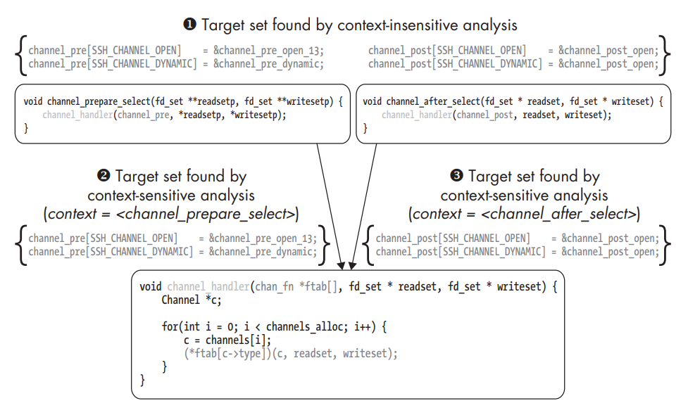 Context-sensitive versus context-insensitive indirect call analysis.
A context-insensitive indirect call analysis concludes that the indirect call in channel_handler could target any function pointer in either the channel_pre table (passed in from channel_prepare_select) or the channel_post table (passed in from channel_after_select). Effectively, it concludes that the set of possible targets is the union of all the possible sets in any path through the program ➊. In contrast, the context-sensitive analysis determines a different target set for each possible context of preceding calls. If channel_handler was invoked by channel_prepare_select, then the only valid targets are those in the channel_pre table that it passes to channel_handler ➋. On the other hand, if channel_handler was called from channel_after_select, then only the targets in channel_post are possible ➌. Context length is 1.
- As with flow-sensitivity, the upside of context-sensitivity is increased precision, while the downside is the greater computational complexity. In addition, context-sensitive analyses must deal with the large amount of state that must be kept to track all the different contexts. Moreover, if there are any recursive functions, the number of possible contexts is infinite, so special measures are needed to deal with these cases. Often, it may not be feasible to create a scalable context-sensitive version of an analysis without resorting to cost and benefit trade-offs such as limiting the context size.
Control-Flow Analysis
A binary analysis that looks at control-flow properties.
Loop Detection
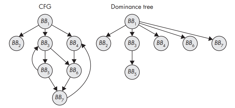 A CFG and the corresponding dominance tree.
- Loops are an interesting target for optimization.
- From a security perspective, analyzing loops is useful because vulnerabilities such as buffer overflows tend to occur in loops.
- Loop detection algorithms used in compilers look for natural loops, which are loops with only 2 blocks that can be said to dominate each other (BB3 and BB5).
- The dominance tree encodes all the dominance relationships in the CFG.
- A basic block A is said to dominate another basic block B if the only way to get to B from the entry point of the CFG is to go through A first. Now a natural loop is induced by a back edge from a basic block B to A, where A dominates B. The loop resulting from this back edge contains all basic blocks dominated by A from which there is a path to B. Conventionally, B itself is excluded from this set. Intuitively, this definition means that natural loops cannot be entered somewhere in the middle but only at a well defined header node. This simplifies the analysis of natural loops.
Cycle Detection
- If a loop can be entered in the middle, then it’s not a natural loop, but a cycle (BB4 to BB7, can be entered at BB6).
- Simply start a depth-first search (DFS) from the entry node of the CFG, then keep a stack where you push any basic block that the DFS traverses and “pop” it back off when the DFS backtracks. If the DFS ever hits a basic block that’s already on the stack, then you’ve found a cycle.
Data-Flow Analysis
A binary analysis that looks at data flow–oriented properties.
Reaching Definitions Analysis
- A data definition can reach a point in the program implies that a value assigned to a variable (or, at a lower level, a register or memory location) can reach that point without the value being overwritten by another assignment in the meantime.
- Reaching definitions analysis is usually applied at the CFG level, though it can also be used interprocedurally.
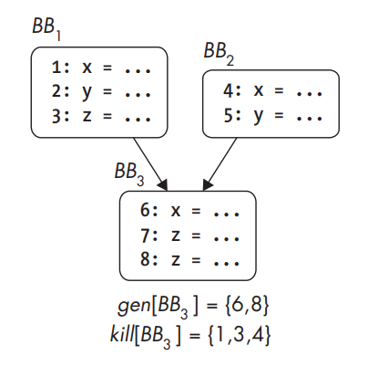 Gen and kill sets for a basic block.
- The analysis starts by considering for each individual basic block which definitions the block generates and which it kills. This is usually expressed by computing a gen and kill set for each basic block. After computing each basic block’s gen and kill sets, you have a local solution that tells you which data definitions each basic block generates and kills. You can compute a global solution that tells you which definitions (from anywhere in the CFG) can reach the start of a basic block and which can still be alive after the basic block.
- The set of definitions reaching B is the union of all sets of definitions leaving other basic blocks that precede B. The set of definitions leaving a basic block B is denoted as out[B] and defined as follows: out[B] = gen[B] ∪ (in[B] − kill[B])
- Since there’s a mutual dependency between the definitions of the in and out sets: in is defined in terms of out, and vice versa, it’s not enough for a reaching definitions analysis to compute the in and out sets for each basic block just once. Instead, the analysis must be iterative: in each iteration, it computes the sets for every basic block, and it continues iterating until there are no more changes in the sets. Once all of the in and out sets have reached a stable state, the analysis is complete.
Use-Def Chains
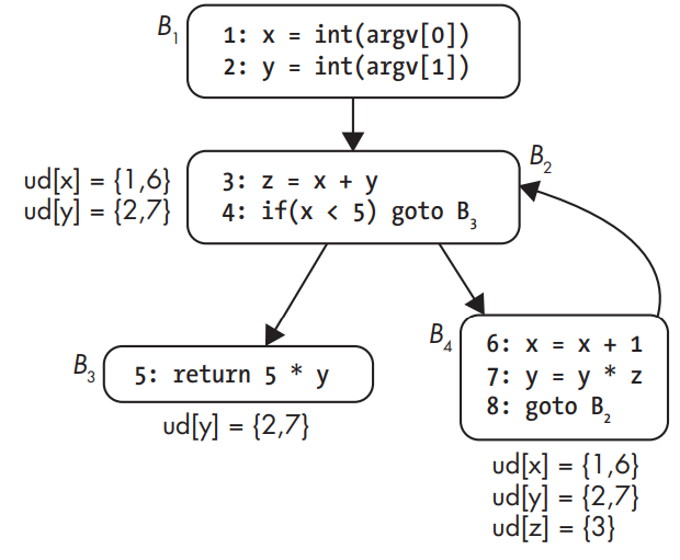 Use-def chains.
- Tell you at each point in the program where a variable is used, where that variable may have been defined.
- Used in decompilation: they allow the decompiler to track where a value used in a conditional jump was compared. This way, the decompiler can take a cmp x,5 and je (jump if equal) instruction and merge them into a higher-level expression like if(x == 5).
- Use-def chains are also used in compiler optimizations such as constant propagation, which replaces a variable by a constant if that’s the only possible value at that point in the program.
The use-def chain for y in B2 contains statements 2 and 7. This is because at that point in the CFG, y could have gotten its value from the original assignment at statement 2 or (after one iteration of the loop) at statement 7. Note that there’s no use-def chain for z in B2, as z is only assigned in that basic block, not used.
Program Slicing
- Aims to extract all instructions (or, for source-based analysis, lines of code) that contribute to the values of a chosen set of variables at a certain point in the program (called the slicing criterion).
- Backward slicing searches backward for lines that affect the chosen slicing criterion.
- Forward slicing starts from a point in the program and then searches forward.
Effects of Compiler Settings on Disassembly
Optimized code is usually significantly harder to accurately disassemble (and therefore analyze). Optimized code corresponds less closely to the original source, making it less intuitive to a human.
- Compilers will go out of their way to avoid the very slow mul and div instructions and instead implement multiplications and divisions using a series of bitshift and add operations.
- Compilers often merge small functions into the larger functions calling them, to avoid the cost of the call instruction; this merging is called inlining.
- Compilers often emit padding bytes between functions and basic blocks to align them at memory addresses where they can be most efficiently accessed. Interpreting these padding bytes as code can cause disassembly errors if the padding bytes aren’t valid instructions.
- Compilers may “unroll” loops to avoid the overhead of jumping to the next iteration. This hinders loop detection algorithms and decompilers, which try to find high-level constructs like while and for loops in the code.
Citation: Practical Binary Analysis.